A benchmark for fluid rigid body interaction with standard CFD packages
Henry von Wahl & Thomas Richter & Jan Heiland
Christoph Lehrenfeld & Piotr Minakowski
GAMM CSE -- 21 November 2019
Introduction
What is a Benchmark
I haven't found a clear definition of what a benchmark is. However, here is what I think makes a numerical example a benchmark
- Common acceptance as a benchmark -- there are other publications that discuss the same setup.
- Practical relevance -- either in applications or as a testing field for numerical algorithms.
- Reliable reference data -- so that others can test their codes and methods against it.
What is a Benchmark
Basically, everything that would motivate a fellow researchers to use the provided setup and data to benchmark their code.
Why Benchmarks
Quantitative assessments, evaluate performance:
We know that this computation correct, but how efficient is it?
Examples:
Why Benchmarks
Qualitive assessments, evaluate confidence:
Are the computations correct?
Example: FEATFLOW CFD Benchmarking project
Note that:
The more complex the model is, the more necessary are benchmarks but the more difficult are benchmark definitions.
Fluid Structure Interaction
- Changing domain.
- Coupling of Models (and scales).
Our Benchmark
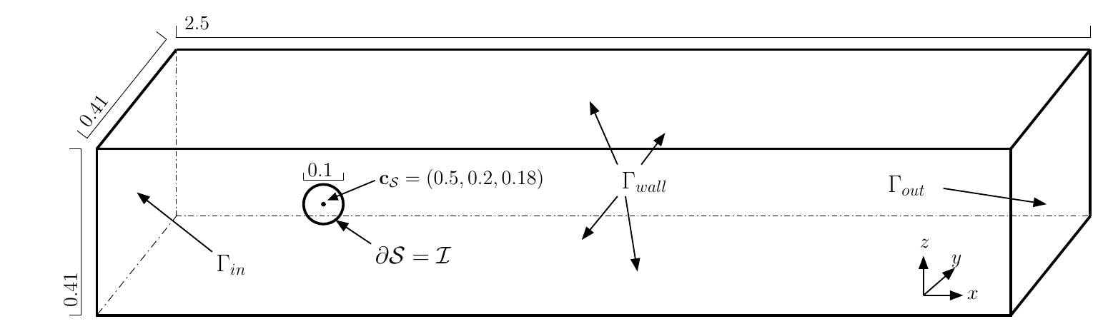
A freely rotating sphere with fixed center
- The domain is fixed.
- Can concentrate on the coupling of the models.
- Accessible to standard CFD solvers.
We address (2.) and (3.) of the benchmark criteria
- Relevant as a testing field for algorithms and
- reliable test data.
(1.) General acceptance as a benchmark may come later.
The model
Verbose
- A fluid flows through a channel with a sphere that can rotate freely.
- The stresses at the sphere/fluid interface induce rotation.
- The no-slip condition induces motion of the flow at the interface.
The flow
\[\begin{equation*} \rho_f\left(\partial_t v + (v \cdot\nabla)v \right) - \nabla \cdot \sigma(v ,p) = 0, \quad \nabla\cdot v = 0, \end{equation*}\] with the stress-tensor \[\begin{equation*} \sigma (v,p) = \rho _ f\nu\left( \nabla v+\nabla v^T \right) - p I \end{equation*}\] and with standard boundary conditions and in particular \[\begin{equation*} v = v_s, \quad \text{on } \mathcal I, \end{equation*}\]where \(v_s\) is the solid's velocity at the fluid-solid interface.
The rigid body
\[\begin{equation*} J\partial_t\omega = \mathbf T \end{equation*}\] where \(J\) is the body's moment of inertia and \(\mathbf T\) is the total torque exerted onto the body by the fluid. \[\begin{equation*} \mathbf T = \int_{\mathcal I} (\mathbf x-\mathbf c)\times \left( \sigma( v,p )\mathbf n \right) ds \end{equation*}\]with the body's centre of mass \(\mathbf c\).
Test Cases
Setups
- 2D and 3D
- stationary -- where there is no torque (low Re-number)
- periodic -- a limit cycle (moderate Re-number)
- time dependent -- a start-up period
how to report the results
To assess the truth the reported data should be
- independent of numerical setup (like the mesh or the scheme),
- dimensionless and suitably parametrized (like through the Reynolds number),
- characteristic for the setup, and
- meaningful for, say, applications.
Characteristic Outputs
for the stationary case
| Variable | Definition |
|---|---|
| \(C_L\) | lift coefficient(s) |
| \(C_D\) | drag coefficient(s) |
| \(C_T\) | torque coefficient(s) |
| \(\Delta_p\) | pressure difference at the cylinder |
| \({\omega}^{ * }\) | dimensionless rotation |
in the periodic case
We used
- the Strouhal number to characterize the frequency,
- minima, maxima of \(C_D\), \(C_L\), \(C_T\), and \(\omega^{ * }\),
- and \(\Delta_p(t^ * )\) -- at the middle of a period.
Implementation
Code Base
There were 5 independent implementations using established libraries:
- Netgen/NGSolve
- FEniCS/dolfin
- Gascoigne
- SciPy
Algorithms
- inf-sup stable and stabilized equal order elements.
- High-order and standard Taylor-Hood (\(P_2-P_1)\) elements.
- Divergence conforming elements.
- Hybrid Discontinous Galerkin methods.
- Implicit/Explicit time integration.
- Most critical: Evaluation of the boundary integrals.
Results
The reported (converged) characteristic outputs ly within certain confidence intervals \(\Delta_I\):
| Test case | Relative size of \(\Delta_I\) | Critical value |
|---|---|---|
| stationary-2D | \(10^{-5}\) | \(C_L\) |
| periodic-2D | \(10^{-3}\) | \(C_T\) |
| time-dep-2D | \(10^{-3}\) | \(C_L\) |
| stationary-3D | (\(1\)), \(10^{-1}\) | \(\omega^ { * }\) |
Discussion
- The 2D simulations gave reliable results.
- Also the stationary 3D case (at least in absolute numbers).
- The time-dependent 3D results were inconclusive.
- We did not include them in the report.
- Conflict with another benchmark property: the numerical setup should be challenging.
Code Availability
Full data sets for the results as well as all implementations can be found at
Conclusion
Conclusion
Benchmarks are valuable for the assessment of numerical models.
- The proposed benchmark may qualify as such because of
- reliable data,
- setup accessible to standard solvers.
I learned: Numerical analysis matters.
References
von Wahl, Henry, Thomas Richter, Christoph Lehrenfeld, Jan Heiland, and Piotr Minakowski. 2019. “Numerical Benchmarking of Fluid-Rigid Body Interactions.” Computers & Fluids. doi:10.1016/j.compfluid.2019.104290.