Introduction

The control of large-dimensional nonlinear dynamical systems is a challenging task because of the

1. system’s size that means a high demand in computational resources
2. and the nonlinearity that adds model inherent complexity to be resolved by the controller.

As long as the system is linear, the computational demands (1.) are well met by powerful and modern linear algebra tools and specialized hardware. A nonlinearity (2.) in small dimensions can be treated through system insights or, sometimes, by repeated linearizations. If nonlinear and large-scale comes together things become tricky.

Here, we try to find the way out by proposing a formulation that is

1. linear by its overall structure
2. with the nonlinearities parametrized by just a few number of parameters.

System approximation by low-dimensional linear parametrizations

In the (nonlinear) Navier-Stokes equations that describe the evolution of fluid flow, the nonlinear term is given by the convection term in the form

$$ f(v) = N(v)\, v $$

where, for any velocity field $v$, the convection operator $N(v)$ describes how the velocity field itself is convected. In a simulation $N(v)$ is a matrix that multiplies the state vector $v$. Despite this matrix structure, the nonlinearity $N(v)\,v$ is deemed complex because $v$ and $N(v)$ are typically very large. If, however, one could approximately (but sufficiently accurately) parametrize $N(v)$ by, say, three scalar parameters $(\rho_1(v), \rho_2(v), \rho_3(v))$ and three basis matrices $N_1$, $N_2$, and $N_3$, i.e.

$$ N(v) \approx \rho_1(v)N_1 + \rho_2(v)N_2 + \rho_3(v)N_3x $$

then the nonlinearity

$$ N(v)\,v \approx \rho_1(v)N_1\,v + \rho_2(v)N_2\,v + \rho_3(v)N_3\,v $$

becomes replaced by a hopefully easy computation of $\rho(v)$ and, notably, just three matrix vector multiplications – the standard operation of numerical linear algebra. And the problem, as we wanted it, appears to be basically linear and only with a low dimensional nonlinearity.

Low-dimensional parametrization of fluid flow

In view of parametrizing $N(v)$, we look for a low-dimensional approximative parametrization of $v$. Low-dimensional approximations of the state of dynamical systems is both the core and promise of classical model order reduction. For our application, however, we would like to trade in some accuracy for very low dimensionality for what classical model reduction techniques are notoriously unsuited.

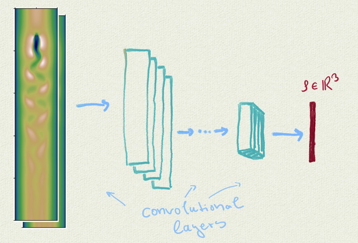
Therefore, we explored how deep convolutional autoencoders (CAEs) could be of help here. CAEs have been developed and successfully used two encode images in a low-dimensional latent feature space for, e.g., classification purposes. For us, the images will be velocity states (as we would plot them, e.g., in Figure 1) and the space of latent features will provide us with a low dimensional parametrization (see Figure 2/3 of an example architecture and an illustration of the dimension reduction).

Apart from providing a flexible and thanks to modern machine learning toolboxes efficiently implementable encoding and decoding mechanism, deep convolutional autoencoders seems a good choice for our tasks as

• by the socalled sparse connectivity the neural network itself requires a moderate number of parameters despite possibly large dimensions of the data
• the implemented operations are shift invariant, meaning a pattern will be detected equally well independent of its position (which seems a good thing to have when thinking of fluid flow)
• the reduction operation of pooling can be seen as providing a multilevel view on the data

Simulation of low-dimensionally parametrized flows

We considered the two dimensional flow behind a round obstacle that develops a periodic shedding of vertices (see Figure 1). In our simulations, we checked if we can indeed replace the $50'000$ dimensional $v$ in $N(v)$ by $\rho(v)$ with literally only $3$ components.

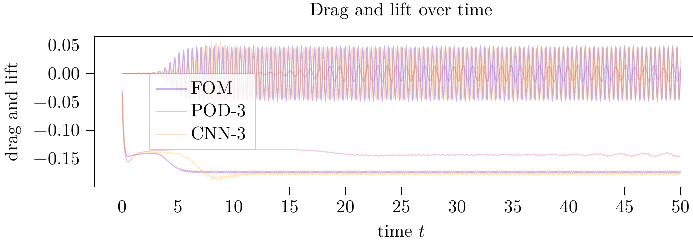
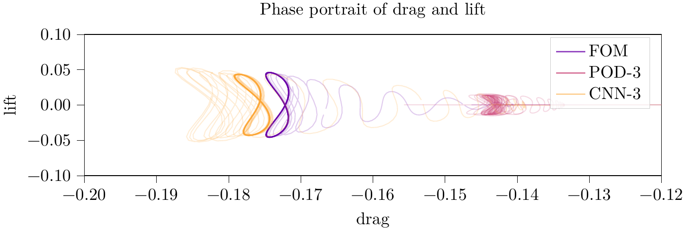
Since in these systems, from a local perspective, small changes can have extreme impacts, differences in the simulation are best evaluated qualitively. Therefore, instead of plotting errors between trajectories (as we did for drag and lift in Figure 4 anyways), we sketched out the phase portrait of how drag and lift that the cylinder experiences evolve in the 2D plane over time.

From Figure 5 we can observe that the CAE approach with 3 parameters well approximates the limit cycle of the full order simulation both in position in size (in particular if compared to the rather standard parametrization approach using POD).

Bibliography

For further reading we recommend our paper that has the detailed theory for this presented example application. A numerical study directed to improve the encoding with the help of clustering can be found in

If you want to redo and expand on the simulations, please check out the codes that accompany the papers.