1 Introduction
Differential-algebraic equations (DAEs) are coupled differential- and algebraic equations. DAEs often describe dynamical processes – here are the differential equations – that are subject to constraints: the algebraic equations.
Let’s start with a few examples.
1.1 Examples
Free fall vs. the pendulum
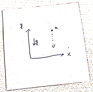
Figure 1.1: Free fall of a point mass.
Here, the laws of the free fall – a special case of Newton’s second law – applies:
force equals mass times acceleration
In 2D, the x, y coordinates of a point of mass m:
m¨x=0m¨y=−mg
where g is the gravity; see Figure 1.1.
The Pendulum
The same point mass attached to a string.
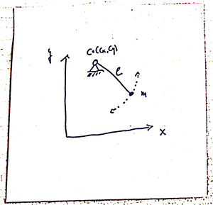
Figure 1.2: A pendulum.
Again, we have force = mass*acceleration but also the conditions that the mass moves on a circle:
(x(t)−cx)2+(y(t)−cy)2=l2, where (cx,cy) are the coordinates of the center and l is the length of the string; see Figure 1.2.
We use the Lagrangian function to derive the Euler-Lagrange equations of motion. For the pendulum, we have the kinetic energy T=12m(˙x(t)2+˙y(t)2), the potential U=mgy, and the constraint h=(x(t)−cx)2+(y(t)−cy)2−l2.
Thus, with L:=U−T−λh and the requirement that ddt(∂L∂˙q)−∂L∂q=0 for all of the generalized coordinates q=x, y, λ, one obtains a system of equations:
| Generalized coordinate | Equation |
|---|---|
| q←x | m¨x(t)+2λ(t)(x(t)−cx)=0 |
| q←y | m¨y(t)−mg+2λ(t)(y(t)−cy)=0 |
| q←λ | (x(t)−cx)2+(y(t)−cy)2−l2=0 |
Example 1.1 (The Pendulum) After an order reduction via the new variables u:=˙x and v=˙y the overall system reads
˙x=u˙y=vm˙u=−2λ(x−cx)m˙v=−2λ(y−cy)+mg0=(x−cx)2+(y−cy)2−l2,
where we have omitted the time dependence.Equation (1.1) is a canonical example for a DAE with combined differential and algebraic equations.
Electrical Circuits
Another class of DAEs arises from the modelling electrical circuits. We consider the example of charging a conductor through a resistor as illustrated in Figure 1.3.
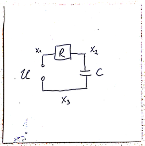
Figure 1.3: Electrical circuit with a source, a resistor, and a conductor.
We formulate the problem in terms of the potentials x1, x2, x3, that are assumed to reside in the wires between a source U and a resistor R, the resistor R and the capacitor C, and the capacitor and the source.
A model for the circuit is given through the following principles and considerations.
| Model principle | Equation |
|---|---|
| The source defines the difference in the neighboring potentials: | x1−x3−U=0 |
| The current IR that is induced by the potentials neighboring the resistor is is defined through Ohm’s law: | IR=x1−x2R |
| The current IC that is induced by the potentials neighboring the capacitor is described through: | IC=C(˙x3−˙x2) |
| Everywhere in the circuit the currents sum up to zero. (This is Kirchhoff’s law): | IC+IR=C(˙x3−˙x2)+x1−x2R=0 |
| To fix the potential, one can set a ground potential – here we choose x3. (note that so far all equations only consider differences in the potential). | x3=0 |
Automatic Modelling or Engineers vs. Mathematicians
If a system, say an engine, consists of many interacting processes, it is convenient and common practice to model the dynamics of each particular process and to couple the subprocesses through interface conditions.
This coupling is done through equating quantities so that the overall model will consist of dynamical equations of the subprocesses and algebraic relations at the interfaces – which makes it a DAE.
In fact, tools like modelica for automatic modelling of complex processes do exactly this.
The approach of automatic modelling is universal and convenient for engineers. However, the resulting model equations will be DAEs which, as we will see, pose particular problems in their analytical and numerical treatment.
1.2 Why are DAEs difficult to treat
Firstly, DAEs do not have the smoothing properties of ODEs, where the solution is one degree smoother than the right hand side. Secondly, the algebraic constraints are essential for the validity of the model. Thus, a numerical approximation may render the model infeasible.
Non-smooth Solutions
Example 1.3 Consider the equation
˙x1(t)=x2(t)0=x2(t)−g(t)
where g can be a nonsmooth function like
g(t)={0,ift<11,ift≥1
In this case the solution part x1=const.+∫t0g(s)ds will be a smooth function and the solution part x2=g will have jumps.Even worse, the solution of a DAE may depend on derivatives of the right hand sides.
This observation indicates that certain difficulties will arise since
- numerical approximation schemes require smoothness of the solutions
- differentiation is numerically ill-posed unlike numerical integration
Numerical Solution Means Approximation
Imagine the equations (1.1) that describe the pendulum are solved approximately. Then, the algebraic constraint will be violated, i.e. the point mass will leave the circle and the obtained numerical solution becomes infeasible.
Thus, special care has to be taken of the algebraic constraints when the equations of motions are numerically integrated.